Visualization

After assembling the dataflow, several visualization features become available to the Driver. Hamilton dataflow visualizations are great for documentation because they are directly derived from the code.

On this page, you’ll learn:

• the available visualization functions

• how to answer lineage questions

• how to apply a custom style to your visualization

For this page, we’ll assume we have the following dataflow and Driver:

# my_dataflow.py
def A() -> int:
    """Constant value 35"""
    return 35

def B(A: int) -> float:
    """Divide A by 3"""
    return A / 3

def C(A: int, B: float) -> float:
    """Square A and multiply by B"""
    return A**2 * B

def D(A: int) -> str:
    """Say `hello` A times"""
    return "hello "

def E(D: str) -> str:
    """Say hello*A world"""
    return D + "world"

# run.py
from hamilton import driver
import my_dataflow

dr = driver.Builder().with_modules(my_dataflow).build()

Available visualizations

View full dataflow

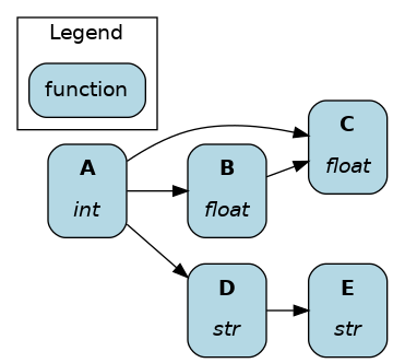
During development and for documentation, it’s most useful to view the full dataflow and all nodes.

dr.display_all_functions(...)

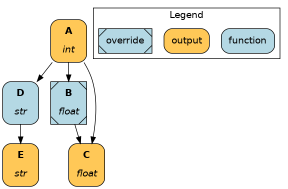
View executed dataflow

Visualizing exactly which nodes were executed is more helpful than viewing the full dataflow when logging driver execution (e.g., ML experiments).

You should produce the visualization before executing the dataflow. Otherwise, the figure won’t be generated if the execution fails first.

# pull variables to ensure .execute() and
# .visualize_execution() receive the same
# arguments
final_vars = ["A", "C", "E"]
inputs = dict()
overrides = dict(B=36.1)

dr.visualize_execution(
    final_vars=final_vars,
    inputs=inputs,
    overrides=overrides,
)
dr.execute(
    final_vars=final_vars,
    inputs=inputs,
    overrides=overrides,
)

An equivalent method is available if you’re using materialization.

materializer =  to.json(
    path="./out.json",
    dependencies=["C", "E"],
    combine=base.DictResult(),
    id="results_to_json",
)
additional_vars = ["A"]
inputs = dict()
overrides = dict(B=36.1)

dr.visualize_materialization(
    materializer,
    additional_vars=additional_vars,
    inputs=inputs,
    overrides=dict(B=36.1),
    output_file_path="dag.png"
)
dr.materialize(
    materializer,
    additional_vars=additional_vars,
    inputs=inputs,
    overrides=dict(B=36.1),
)

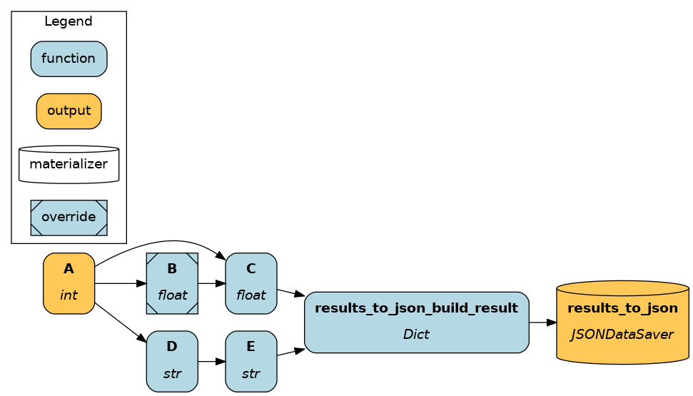
Learn more about Materialization.

View node dependencies

Representing data pipelines, ML experiments, or LLM applications as a dataflow helps reason about the dependencies between operations. The Hamilton Driver has the following utilities to select and return a list of nodes (to learn more Lineage + Hamilton):

• .what_is_upstream_of(*node_names: str)

• .what_is_downstream_of(*node_names: str)

• .what_is_the_path_between(upstream_node_name: str, downstream_node_name: str)

These functions are wrapped into their visualization counterparts:

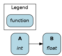
Display ancestors of B:

dr.display_upstream(["B"])

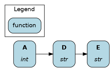
Display descendants of D and its immediate parents (A only).

dr.display_downstream(["D"])

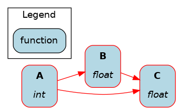
Filter nodes to the necessary path:

dr.visualize_path-between("A", "C")
# dr.visualize_path-between("C", "D") would return
# ValueError: No path found between C and D.

Configure your visualization

All of the above visualization functions share parameters to customize the visualization (e.g., hide legend, hide inputs). Learn more by reviewing the API reference for Driver.display_all_functions(); parameters should apply to all other visualizations.

Apply custom style

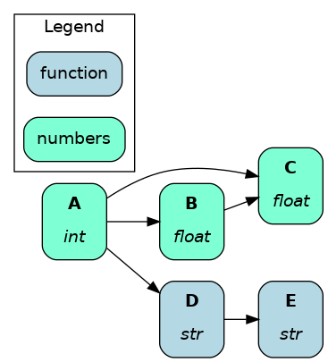
By default, each node is labeled with name and type, and stylized (shape, color, outline, etc.). By passing a function to the parameter custom_style_function, you can customize the node style based on its attributes. This pairs nicely with the @tag function modifier (learn more Add metadata to a node)

Your own custom style function must:

1. Use only keyword arguments, taking in node and node_class.

2. Return a tuple (style, node_class, legend_name) where:

   • style: dictionary of valid graphviz node style attributes.

   • node_class: class used to style the default visualization - we recommend returning the input node_class

   • legend_name: text to display in the legend. Return None for no legend entry.

3. For the execution-focused visualizations, your custom styles are applied before the modifiers for outputs and overrides are applied.

If you need more customization, we suggest getting the graphviz object produced, and modifying it directly.

This online graphviz editor can help you get started!

def custom_style(
    *, node: graph_types.HamiltonNode, node_class: str
) -> Tuple[dict, Optional[str], Optional[str]]:
    """Custom style function for the visualization.

    :param node: node that Hamilton is styling.
    :param node_class: class used to style the default visualization
    :return: a triple of (style, node_class, legend_name)
    """
    if node.type in [float, int]:
        style = ({"fillcolor": "aquamarine"}, node_class, "numbers")

    else:
        style = ({}, node_class, None)

    return style

dr.display_all_functions(custom_style_function=custom_style)

See the full code example for more details.